[NUMERICAL ANALYSIS] Using XLSLANI's RK4 and RKF45 to solve differential equations

Hi! For the first guide, it's how to solve a system of ordinary differential equations using XLSLANI. Actually, one of the main reasons why the addin is developed is because of the near non-existence of non-paywalled numerical solvers for ODE.

Actually, there's Octave. But Excel is more easily accessible over Octave, and if you want quick ODE solving, you aren't looking for something like Octave, you're looking for something quick enough to access like Polymath. But Polymath has a paywall, so...

Anwyay, to start, say we have these two chemical reactions ongoing.

If we treat them as elementary chemical reactions, we have these three differential equations.

We note that CA starts at 5.0 M, CR starts at 0.1 M, and there is no CR, if we want the transient concentrations of the reaction we have to integrate the set of differential equations. We want to determine the behavior of the reaction from t = 0 to t = 5. 

In the spreadsheet, we can write dCA/dt, dCR/dt, and dCS/dt to make looking at the spreadsheet easier (I don't easily get confused when looking at spreadsheets with large amounts of numbers sprawling on it, but for the sake of tutorial, we do this). Also, we can write t(i) and t(f) to denote the initial and final integration; and CA(0), CR(0), and CS(0) to denote the initial concentrations. Then, we begin by writing the differential equations. 

In writing the differential equations, CA is selected as CA(0), CR as CR(0), and CS as CS(0) in representing the variables of the ODE. I pressed the [Show Formulas] button in Excel so my action is made clear.

As it can be seen, in the differential equations, CA is assigned cell F11, where CA(0) lies, and CR is assigned F12, where CR(0) lies. There is no CS which is theoretically supposed to be F13 (the cell for CS(0), as there is no CS in the system of ODE.

We then plug in our initial and final time, as well as the initial conditions for the ODE system. The spreadsheet should look something like this:

Those evaluations are actually the k1 evaluations for a Runge-Kutta approach of solving ODE. Actually it also serves the purpose that one can compare the initial ODE evaluations to determine if the system ODEs is a stiff set of ODEs (you know, where one of the differential equations evaluate to around 0.1, then the others evaluate to orders of tens or hundreds in magnitude, something like 1000 ot 10000). If the ODE set is stiff, use of the traditional Runge-Kutta and Euler is not advisable as you would need practically microscopic steps just to propagate your solution.

Anwyay that's enough rambling. Clearly, this is NOT a stiff equation, so we use the traditional fourth-order Runge-Kutta. Anyway, the formula is here, courtesy of Dr. Pestaño's numerical analysis notes:

A/N: For the curious chemical engineer reading this, yep. That dCR/dt is essentially the same dCR/dt as to what I wrote there, even though she reworded the problem differently (probably as to not confuse people, she typically teaches nice such that you are able to understand everything at your own pace which is lovable, then she will try to kill you later in the exam 😂). Actually, when she taught us Kinetics, that ODE appeared again but we were solving the original formulation (the one that I first wrote) in an analytic and numeric hybrid approach.

Alright. So how do we solve the system of ODE using the spreadsheet?

First, we highlight some m rows by n columns in the spreadsheet. As to the amount of columns, it must be equivalent to the number of columns plus one; the plus one is due to the independent variable column which sits at the first column. So in our case, we need to highlight exactly four columns. For rows however, is for you to decide which I shall elaborate later. For now just... highlight at least say, 20 rows. So that would be a 20x4 array.

By the way, I wrote the variables there so as to not confuse the person reading this. This should also show the order of arrangement of the variables in the ODE solution. From there, we begin our ODE solution.

We type the following:

=XLSLANI_RK4(F4:F6,F8,F9,F11:F13,15)

• F4:F6 denote the range where the differential equations are.
• F8 denotes the initial value of the independent variable (time)
• F9 denotes the final value of the independent variable (again, time)
• F11:F13 denote the range where the initial value for each of the variables in the differential equations are.
• What is 15? This means that the solver will solve for 15 times (basically, this is telling it that the number of segments from 0 to 5 is 15. This means the resulting stepsize is (5 - 0) / 15 = 0.33333.
• Wait - but we highlighted 20 rows. This means that the solver will basically ignore the other rows and put #N/A there instead. This is what I meant earlier by putting whatever amount of rows there. Just put many so that the entire result table will be printed out.

It should look something like this:

Then to get the solution, we just hit the following key combination: CTRL + SHIFT + ENTER. This allows Excel to evaluate the formula in an array fashion. It should print out the results.

There, that's the data for the numerical solution of the ODE. As seen from the resulting table;

CA(5) = 1.432 M; CR(5) = 0.959 M, and CS(5) = 1.354 M.

We can also highlight everything and enjoy the pretty graph:

Say for example we want to determine t = 50. Substituting 50 there will cause everything to result to a #VALUE! error. 

Why? Basically because the stepsize is too big. h = (50 - 0) / 15 = 3.333; the effective stepsize is 3.333, and that's quite big for the differential equation. So how do we determine the best stepsize? Oversimplifying things, that's an entire field in mathematics (numerical differential equations, it's actually a course in MS Mathematics). 

Just make sure that the resulting stepsize is small enough for the solution not to 'explode', and we can do that in the program by making sure that the segment number is big enough (which is represented by 15 in there). This is oversimplifying the explanation, as to not make your head equally explode like your exploded iteration, or whatever remains of it 😂

If we change it to say, 100; we get this (you would need to re-hit CTRL + SHIFT + ENTER by the way).

Obviously, the highlighted array is not sufficient to show everything. As I said earlier, just highlight blah amount of rows, which I shall be doing, just to show all the data.

Again, I have no idea how many rows I highlighted, I just made sure that the entire iteration table will fit as MS Excel will compensate by putting #N/A anyway. I also adjusted the range of the graph.

Another way to evade the entire 'I-have-no-idea-what-my-stepsize-should-be' issue is to use an adaptive integrator. Basically, this calls for using two Runge-Kuttas of different order, then you compare the two solutions, then if the solutions are too far from each other, you reduce the stepsize such that the two solutions look alike now. This also means that if the function varies too much, most likely the stepsize will be very small, and if not, the steps should be big. 

I have placed the Dormand-Prince/Runge-Kutta-Fehlberg there for this purpose. This is also famously known as the ode45 routine in MATLAB/Octave and RKF45 routine in Polymath (the default ODE solvers). The solver is represented by:

=XLSLANI_RKF45(...)

It has the same input parameters as ODE_RK4, but as the adaptive integration scheme causes the stepsize to vary, it does not guarantee that the amount placed there will result to the final values being calculated (what? I'll show it later). 

Running the RKF45 using the same initial parameter entries;

=XLSLANI_RKF45(F4:F6,F8,F9,F11:F13,15)

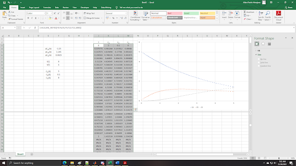
As it can be seen, this is what I meant earlier. Basically the solver only did 15 iterations and printed whatever the result is in the spreadsheet. Unlike RK4 which uses a constant stepsize, RKF45 kept on adjusting the stepsize such that it provides an accurate solution to maximum allowable error ɛ = 0.1 (the default value). So if we want to propagate the solution more, we have to increase both the number of iterations and number of rows by a  blah amount (again excesses does not matter as Excel will just pad #N/A on it, and is totally harmless). Doing some 1000 iterations and I have no idea how many rows this is, results to:

I split the screen so that the end of iterations can be seen; where as seen the iterations did not finish the 1000 iteration requirement I placed, and instead terminated the iterations exactly at t = 5 (interpolation was done at the final iterations). Also, I changed the graph where I showed that the stepsizes are smaller at the more-varying parts of the graph, and wider at the lesser-varying parts.

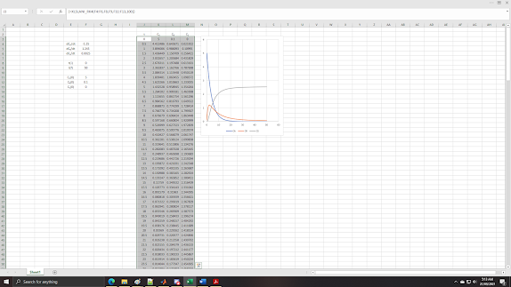
If we do t = 50 again, obviously this solver will fare better:

As it can be seen, it we still did not finish the entire 1000 iterations, but clearly the solution fared better as the solution adjusted to small time steps at smaller values of t (where most of the reactions are taking place) and larger steps at larger values of t (where there is practically nothing happening anymore). To make a traditional method like RK4 work here would require small values of timesteps all throughout. Yay for adaptive integration! ☝

Anyway, optional inputs for XLSLANI_RKF45 can also be inputted such as modifying the minimum and maximum timesteps, and most especially the error tolerance between the two RK's being compared by the adaptive routine.

So that's for the first tutorial. I leave you with that 😝